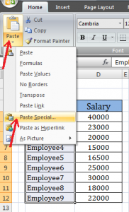
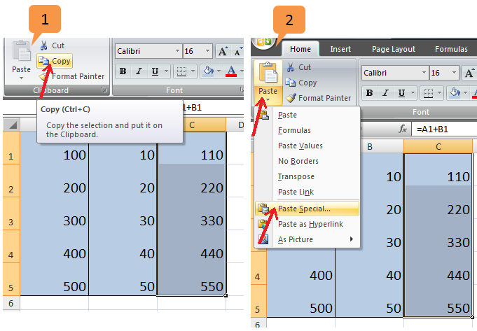
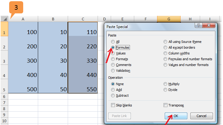
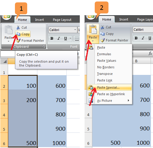
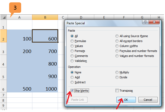
We use copy paste (Ctrl+C and Ctrl+V) commonly to copy data. But surprisingly, there are 17 different variations to paste data in an excel sheet! To Paste Special click on arrow below Paste and click Paste Special.
Hit Alt + E (Edit) followed by S (Paste Special) to display the paste special box. Select the appropriate options in the box.
Steps to Use Paste Special
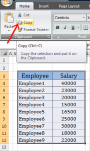
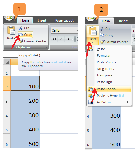
 Select the data to be copied and click Copy on Home tab.

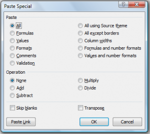
 To Paste Special, select the destination and click the arrow below Paste button on Home tab. Click Paste Special on the drop-down menu. A Paste Special dialog box appears.


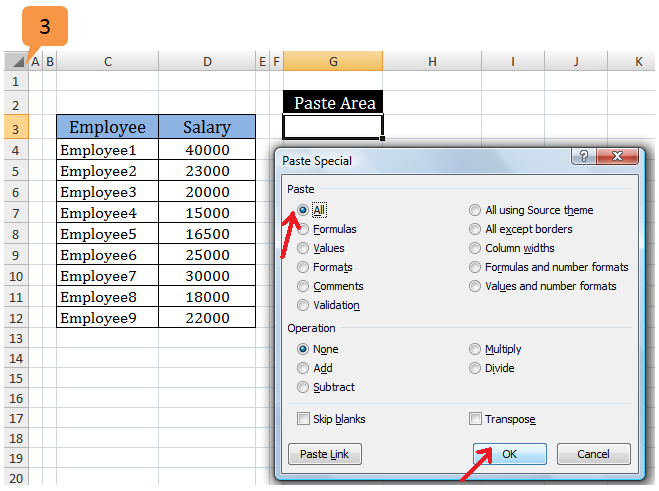
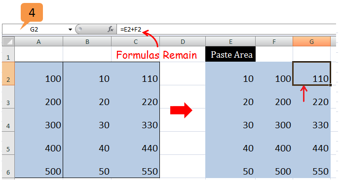
Select appropriate options in the dialogue box.

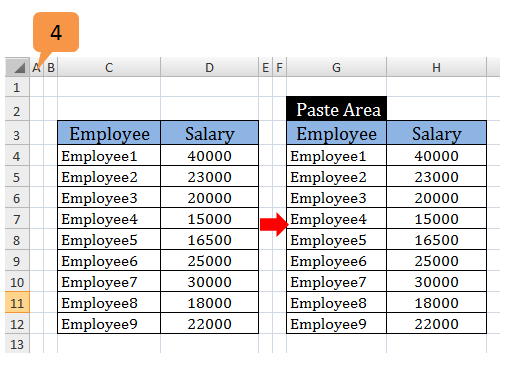
Pastes everything (formulas, formatting, and text) . (Same as Paste).
Shortcut: Hit Alt + E (Edit) followed by S (Paste Special) and A (All) or simply Ctrl + V.


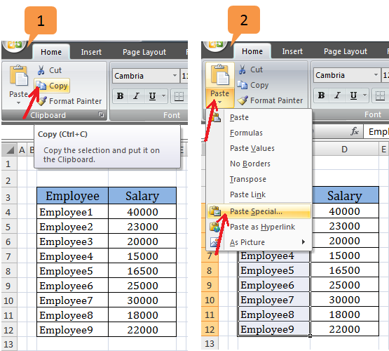
It enables pasting just the formulas ignoring everything else. This is useful, because it retains the formatting and comments of the destination cells.
Shortcut: Hit Alt + E (Edit) followed by S (Paste Special) and F (Formulas).


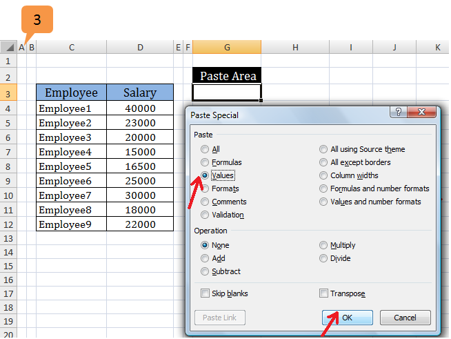
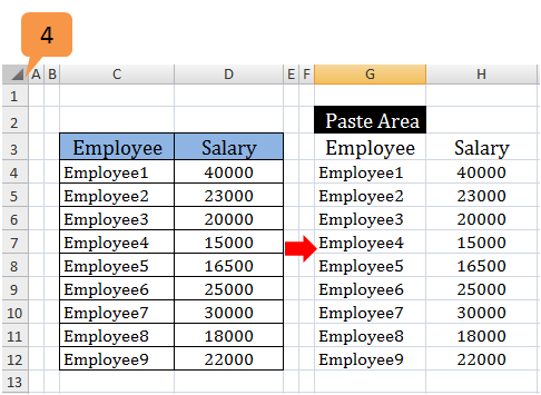
It Pastes only values without formatting. It doesn’t matter if the source cell has a formula in it. If you wish to paste data from one worksheet to another that contains links, this option is useful to
avoid links to another file.
Shortcut: Hit Alt + E (Edit) followed by S (Paste Special) and V (Values).


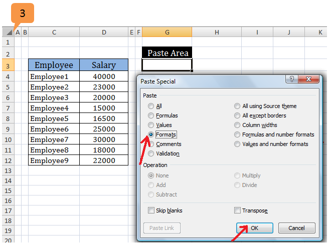
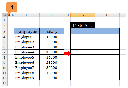
This option enables to paste only the formatting (and conditional formatting) from the copied cells to destination cells. This is useful if you have content formatted in a certain way that you would like to copy to another location.
Shortcut: Hit Alt + E (Edit) followed by S (Paste Special) and T (Formats).


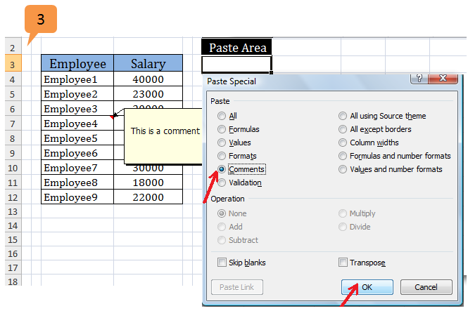
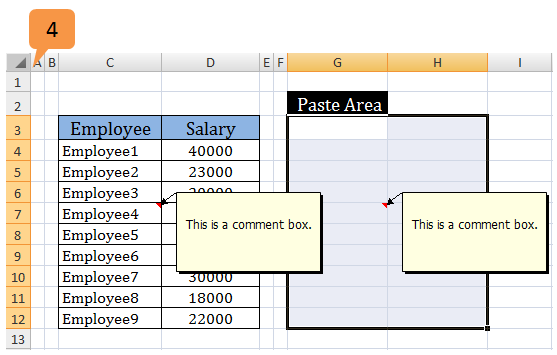
This option enables pasting only comments from the copied cell to the new cell, without pasting any of the formats or data from the source cell. This option saves you the time of re-typing comments, while preserving the data and formats in the destination cell.
Shortcut: Hit Alt + E (Edit) followed by S (Paste Special) and C (Comments).


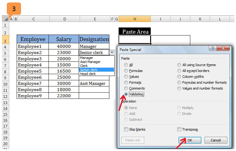
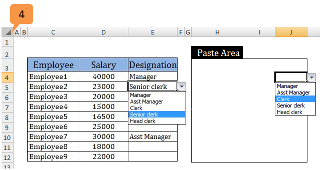
When creating Data Validation rules, you might want to apply those rules to other cells. You can do that with this option without copying any source data or formats, and preserving the destination data and formats.
Shortcut: Hit Alt + E (Edit) followed by S (Paste Special) and N (Validation).


 All using Source theme:
This option pastes all the information from the source cell (numbers, formulas, text, formats, comments, etc.) and applies the source worksheets theme’s colors, fonts and graphics to the destination.
 All except borders:
This option pastes numbers, formulas, text, comments and formats except borders from the source cell in the destination cell.
 Column widths:
It allows you to copy one column’s width or more and apply it to whichever columns you select. If your spreadsheet has one wide column of data, and you want that wide column look normal, select the normal column and paste Column Width, so that all columns are of equal width.
 Formulas and number formats:
This option pastes only the formula from the source cell and number formats applied to that cell. It only pastes number formatting, such as percentage, currency, accounting, scientific, etc., and other formats like border, fill color, font, etc., are not pasted.
 Values and number formats:
This option pastes the same information as the Formulas and number formats option above, except it only pastes values and not formulas. This is similar to the Values option discussed above with the addition of the number formatting.
Operation Section
The Operation section allows you to perform a mathematical operation with the data you have copied.
For example, let us assume that a source cell contains number 5, and the destination cell contains number 10.
Let us assume that the “All” option is selected from the Paste section with Skip blanks and Transpose left unchecked.
Below are the results of each operation option
 None:
None:
This operation performs no arithmetic, and therefore resulting number in the destination cell will be 5.
 Add:
Add:
By selecting 5 from the source cell and pasting it into the destination, which contains 10, Excel adds 10+5 to return 15.
 Subtract:
Excel subtracts 10-5 to return 5.
 Multiply:
Excel multiplies 10*5 to return 50.
 Divide:
Excel divides 10/5 to return 2.
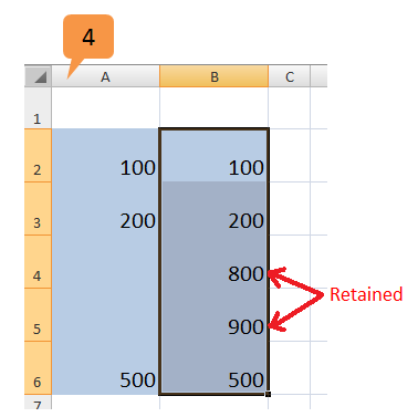
There are three more options on the menu: Skip blanks, Transpose and Paste Link.

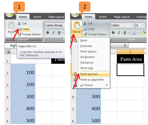
This option works just as it says. The Skip blanks option tells Excel to paste only where there is data in the source cell. If the cells are blank, Excel will skip over them and not paste anything, which is why cells B4 and B5 had the values of 800 and 900 respectively instead of being blank.


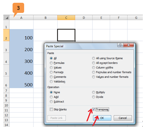
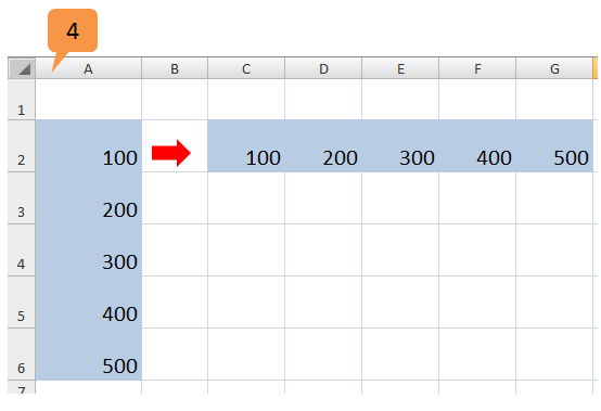
The Transpose option takes a copied list of numbers from a column and pastes them across a row, or copies a list of numbers from a row and pastes them down a column.


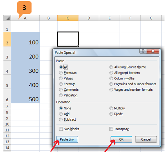
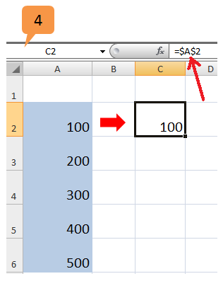
If you want your destination cell to link to the source cell you can use this option. In cell C2, you can see the formula ‘=$A$2’. If you select multiple cells to paste, it won’t have the dollar($) signs. Paste Link option saves a lot of time if you’re working with multiple worksheets or multiple files.


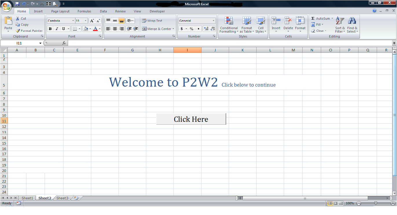

 Hide sheet tabs.
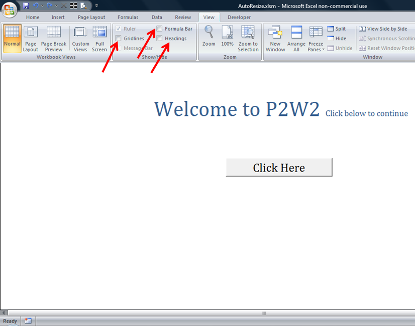
 Remove Grid Lines, Headings and hide Formula Bar.
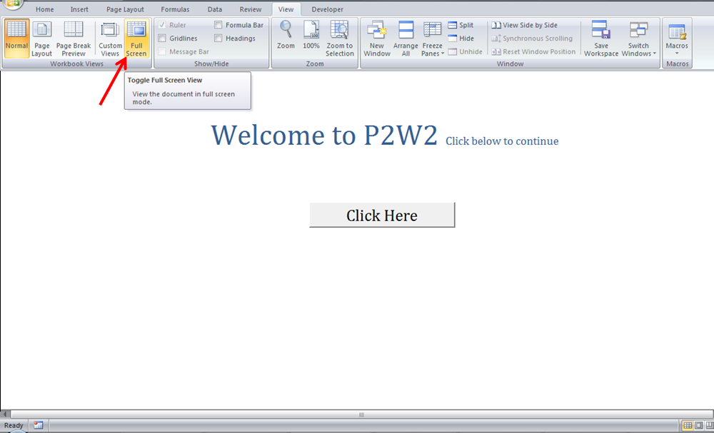
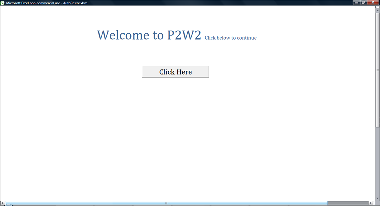
 Select Excel ‘Full Screen’ option from ‘View’ menu.
 Hide sheet tabs.
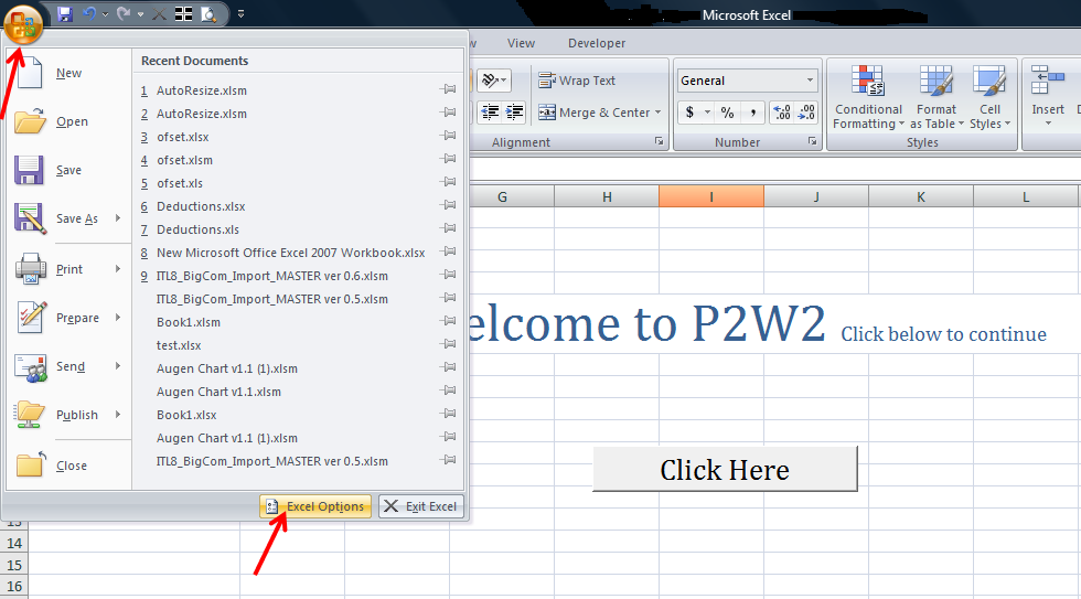
 Select ‘Office’ Button and select ‘Excel Options’.
 Select ‘Advanced’ option under ‘Display Options for This Workbook’ uncheck the box ‘Show Sheet Tabs’.
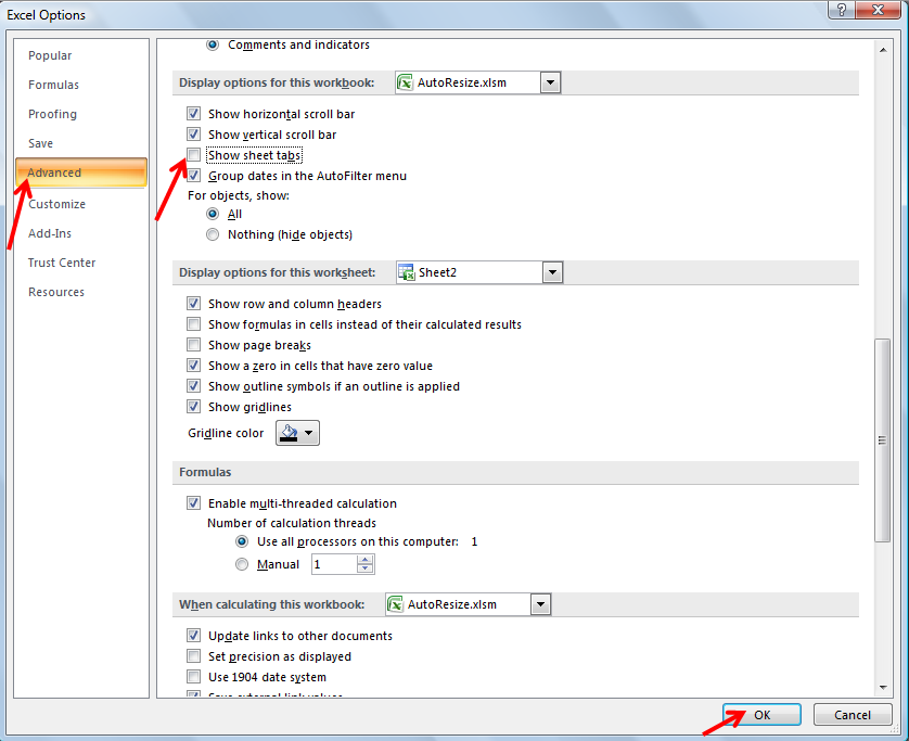
 Click ‘Ok’.
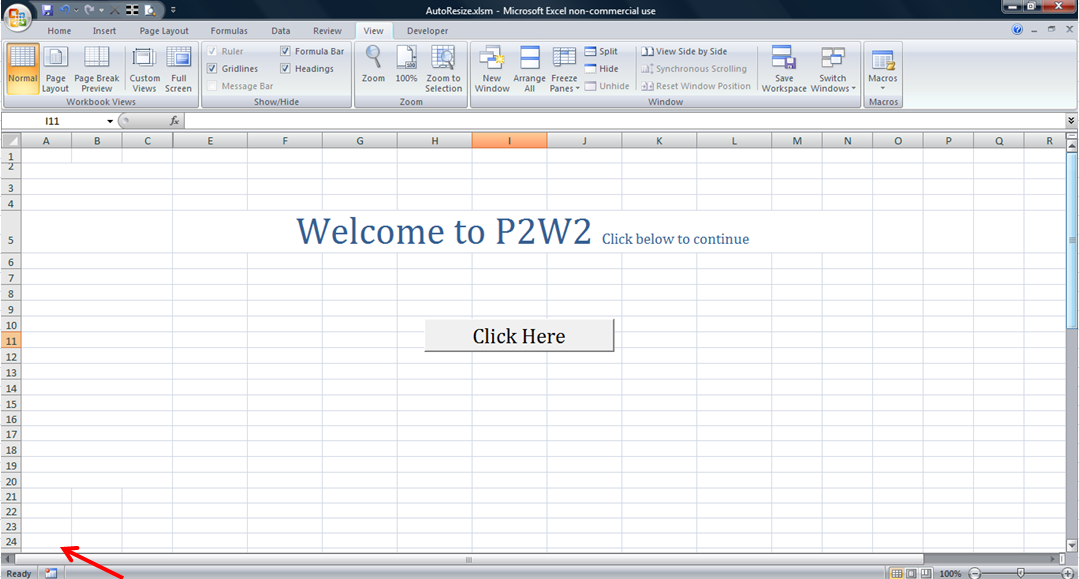
 Removing Grid lines, Headings and Formula Bar.
 Selecting Excel Full Screen