How to Avoid Screen Updating in Excel VBA?

This article helps to handle the screen updates using macro. We can speed up our macro by turning off the screen updating while the macro runs, by adding the below line of code to the macro:
Sub Macro ()
Application.ScreenUpdating = False

Write the necessary code Here

——————-

——————-
Application.ScreenUpdating = True
End Sub.

The prior versions of excel 2000, it was not

required to turn ScreenUpdating back to

true. When the macro is finished, Excel would revert back to turning the screen updating to true.

But now whether you are writing macros in Excel 97, Excel 2000, Excel 2002, 2003, 2007 or 2010 always we have to turn the screen updating back to true with the below code:
Application.ScreenUpdating = True

Vani is a Business Associate with p2w2, a Spreadsheet Solutions company. p2w2 has expertise in Excel Modeling, Excel Dashboards, Profitability Analysis, Excel Invoicesand Excel Bid sheets. You can contact us by email: cs [at] p2w2.com or call us at 305.600.0950.

How to do a Two-Way Lookup in Excel?

Excel spreadsheets support lookup functions that return a value from a table by looking up another value in the table. The vlookup and hlookup functions in Excel work as one-way lookups. This article helps you to perform a two way lookup.

The Pi

cture below shows a simple example:

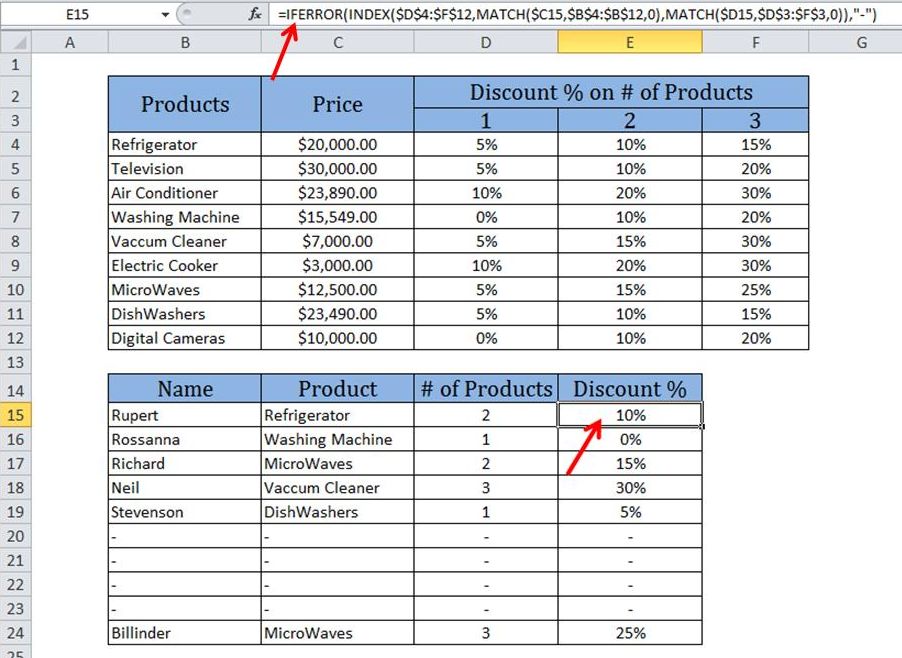
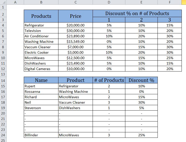
The first table shows products, Price of the product and discount on number of products purchased. The second table shows name of the person, product purchased, number of products purchased and discount applicable.

A formula is used in column E of second table to get the discount percentage from the first table as shown in the picture below:

The formula in cell E15 looks up the values of cells C15(Product) and D15(# of Products) in the first table and returns the corresponding value from the table.

The formula in E15 is:

=IFERROR(INDEX($D$4:$F$12,MATCH($C15,$B$4:$B$12,0),MATCH($D15,$D$3:$F$3,0)),”-“)

Description of the formula:

The above formula uses the INDEX function, which consists of three arguments.

The first argument gives the entire range of ‘Discount% on # of products’ from first table($D$4:$F$12).

=IFERROR(INDEX($D$4:$F$12,MATCH($C15,$B$4:$B$12,0),MATCH($D15,$D$3:$F$3,0)),”-“)

The second argument is MATCH function. MATCH ($C15,$B$4:$B$12,0)

It matches the ‘product’ in cell C15 of second

table with the ‘products’ in cells B4 to B12 of first table and returns the ‘Product.

=IFERROR(INDEX($D$4:$F$12,MATCH($C15,$B$4:$B$12,0),MATCH($D15,$D$3:$F$3,0)),”-“)

The third argument is also a MATCH function. MATCH ($D15,$D$3:$F$3,0).

It matches the ‘# of products’ in cell D15 of second table with the ‘Discount% on # of products’

in cells D3 to F3 of first table and returns the ‘# of products’.

=IFERROR(INDEX($D$4:$F$12,MATCH($C15,$B$4:$B$12,0),MATCH($D15,$D$3:$F$3,0)),”-“).

In this way the above formula is used as a two way lookup formula to retrieve the value required.


How to get a "Print PDF" Button in Excel?

<div>One of the features in Excel is the ability to convert Excel files to PDF format. In this article we explain how to create a button in the excel worksheet, which when clicked generates a PDF file of that sheet.</div>
<div>Let us take the picture below as example to take a PDF and save it in current folder.</div>
<div style=”text-align: center;”><img class=”aligncenter size-full wp-image-1187″ title=”Selected file for PDF” src=”http://www.p2w2.com/blog/wp-content/uploads/2011/11/Selected-file-for-PDF.png” alt=”” width=”550″ height=”230″ /></div>
<h3>Below are the steps to get a button, which converts the excel file to a PDF file:</h3>
<h5><img class=”alignnone size-full wp-image-1188″ title=”1″ src=”http://www.p2w2.com/blog/wp-content/uploads/2011/11/1.png” alt=”” width=”46″ height=”45″ align=”middle” /> <span style=”font-size: 14px; font-weight: normal;”>Select </span><strong style=”font-size: 14px;”>Developer</strong><span style=”font-size: 14px; font-weight: normal;”>, select </span><strong style=”font-size: 14px;”>Insert</strong><span style=”font-size: 14px; font-weight: normal;”> from </span><strong style=”font-size: 14px;”>Control</strong><span style=”font-size: 14px; font-weight: normal;”> group and select </span><strong style=”font-size: 14px;”>Button</strong><span style=”font-size: 14px; font-weight: normal;”> from </span><strong style=”font-size: 14px;”>Form Controls</strong><span style=”font-size: 14px; font-weight: normal;”>.</span></h5>
<div><img class=”aligncenter size-full wp-image-1189″ title=”Insert Button” src=”http://www.p2w2.com/blog/wp-content/uploads/2011/11/Insert-Button.png” alt=””

width=”331″ height=”184″ /></div>
<h5><img class=”alignnone size-full wp-image-1190″ title=”2″ src=”http://www.p2w2.com/blog/wp-content/uploads/2011/11/2.png” alt=”” width=”46″ height=”45″ align=”middle” /> <span style=”font-size: 15px; font-weight: normal;”>Drag the control on the spreadsheet, a window appears.</span></h5>
<h5><img class=”alignnone size-full wp-image-1191″ title=”3″ src=”http://www.p2w2.com/blog/wp-content/uploads/2011/11/3.png” alt=”” width=”46″ height=”45″ align=”middle” /> <span style=”font-size: 14px; font-weight: normal;”>Enter the name of the macro in the tab provided for </span><strong style=”font-size: 14px;”>Macro name</strong><span style=”font-size: 14px; font-weight: normal;”> and click </span><strong style=”font-size: 14px;”>OK</strong><span style=”font-size: 14px; font-weight: normal;”>.</span></h5>
<div><img class=”aligncenter size-full wp-image-1199″ title=”Assign Macro” src=”http://www.p2w2.com/blog/wp-content/uploads/2011/11/Assign-Macro.png” alt=”” width=”381″ height=”366″ /></div>
<h5><img class=”alignnone size-full wp-image-1192″ title=”4″ src=”http://www.p2w2.com/blog/wp-content/uploads/2011/11/4.png” alt=”” width=”46″ height=”45″ align=”middle” /> <span style=”font-size: 14px; font-weight: normal;”>To edit the name of the button, Right click on the button and select </span><strong style=”font-size: 14px;”>Edit Text</strong><span style=”font-size: 14px; font-weight: normal;”>.</span></h5>
<div><span style=”font-size: 14px; font-weight: normal;”><img class=”aligncenter size-full wp-image-1200″ title=”Edit Text” src=”http://www.p2w2.com/blog/wp-content/uploads/2011/11/Edit-Text.png” alt=”” width=”293″ height=”233″ /> </span></div>
<h5><img class=”alignnone size-full wp-image-1193″ title=”5″ src=”http://www.p2w2.com/blog/wp-content/uploads/2011/11/5.png” alt=”” width=”46″ height=”45″ align=”middle” /> <span style=”font-size: 14px; font-weight: normal;”>Right click on the button and select </span><strong style=”font-size: 14px;”>Assign Macro</strong><span style=”font-size: 14px; font-weight: normal;”>.</span></h5>
<div><span style=”font-size: 14px; font-weight: normal;”><img class=”aligncenter size-full wp-image-1201″ title=”Assign Macro” src=”http://www.p2w2.com/blog/wp-content/uploads/2011/11/Assign-Macro1.png” alt=”” width=”381″ height=”366″ />
</span></div>
<h5><img class=”alignnone size-full wp-image-1194″ title=”6″ src=”http://www.p2w2.com/blog/wp-content/uploads/2011/11/6.png” alt=”” width=”46″ height=”45″ align=”middle” /> <span style=”font-size: 14px; font-weight: normal;”>Select the </span><strong style=”font-size: 14px;”>Macro name</strong><span style=”font-size: 14px; font-weight: normal;”> and select </span><strong style=”font-size: 14px;”>New</strong><span style=”font-size: 14px; font-weight: normal;”>.</span></h5>
<div><span style=”font-size: 14px; font-weight: normal;”><img class=”aligncenter size-full wp-image-1202″ title=”Assign New Macro” src=”http://www.p2w2.com/blog/wp-content/uploads/2011/11/Assign-New-Macro.png” alt=”” width=”391″ height=”373″ />
</span></div>
<h5><img class=”alignnone size-full wp-image-1195″ title=”7″ src=”http://www.p2w2.com/blog/wp-content/uploads/2011/11/7.png” alt=”” width=”46″ height=”45″ align=”middle” /> <span style=”font-size: 14px; font-weight: normal;”>A Microsoft Visual Basic window appears.</span></h5>
<div style=”text-align: center;”><span style=”font-size: 14px; font-weight: normal;”><img class=”aligncenter size-full wp-image-1209″ title=”Visual Basic Application” src=”http://www.p2w2.com/blog/wp-content/uploads/2011/11/Visual-Basic-Application2.png” alt=”” width=”539″ height=”262″ />
</span></div>
<h5><img class=”alignnone size-full wp-image-1196″ title=”8″ src=”http://www.p2w2.com/blog/wp-content/uploads/2011/11/8.png” alt=”” width=”46″ height=”45″ align=”middle” /> <span style=”font-size: 14px; font-weight: normal;”>Enter the below code in the application where the arrow is pointed, under ‘</span><strong style=”font-size: 14px;”>Sub CreatePDF()’.</strong></h5>
<blockquote>
<div>Sub CreatePDF()</div>
<div>ActiveSheet.ExportAsFixedFormat Type:=xlTypePDF, Filename:= _</div>
<div>”Generate Report.pdf”, Quality:=xlQualityStandard, _</div>
<div>IncludeDocProperties:=True, IgnorePrintAreas:=False, OpenAfterPublish:= False</div>
<div>End Sub</div></blockquote>
<div style=”text-align: center;”><img class=”aligncenter size-full wp-image-1205″ title=”Code to Generate PDF” src=”http://www.p2w2.com/blog/wp-content/uploads/2011/11/Code-to-Generate-PDF.png”

alt=”” width=”600″ height=”200″ /></div>
<h5><img class=”alignnone size-full wp-image-1197″ style=”font-size: 11px; font-weight: bold;” title=”9″ src=”http://www.p2w2.com/blog/wp-content/uploads/2011/11/9.png” alt=”” width=”46″ height=”45″ align=”middle” /> <span style=”font-size: 14px; font-weight: normal;”>Close the Microsoft Visual Basic application, now just click on the </span><strong style=”font-size: 14px;”>CreatePDF</strong><span style=”font-size: 14px; font-weight: normal;”> button. That’s all a PDF will be generated and saved in the same folder.</span></h5>
<h5><img class=”alignnone size-full wp-image-1206″ title=”10″ src=”http://www.p2w2.com/blog/wp-content/uploads/2011/11/101.png” alt=”” width=”50″ height=”45″ align=”middle” /> <span style=”font-size: 14px; font-weight: normal;”>If we want to change the name of the PDF, we can change it in the code. For example in the second line we have “Generate Report.pdf”, change it to “</span><strong style=”font-size: 14px;”>Create Report.pdf</strong><span style=”font-size: 14px; font-weight: normal;”>”.</span></h5>
<div></div>
<div><strong>————————————————————————————————————–</strong></div>
<strong>
<div>Vani is a Business Associate with p2w2, a Spreadsheet Solutions company. p2w2 has expertise in <a href=”../../chaitanya_sagar/”>Excel Modeling</a>, <a href=”../../excel-dashboard-reporting.php”>Excel Dashboards</a>, <a href=”../../cost-profitability-analysis.php”>Profitability Analysis</a>,  <a href=”../../custom-invoices.php”>Excel Invoices</a>and <a href=”../../custom-invoices.php”>Excel Bid sheets</a>. You can contact us by email: cs [at] p2w2.com or call us at 305.600.0950.</div>
</strong>
<div></div>

free copy of text your ex backhow to win back your ex girlfriend quickly How To Make Your Ex Girlfriend Want You Back Quickly we just spoke after breaking up what nexthow to make your ex want you

How to Sort in Excel?

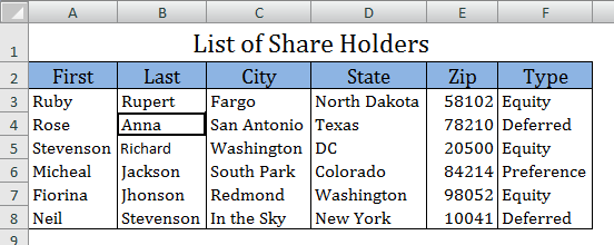
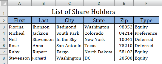
Sorting is used to reorder our data in excel. We can easily reorder the data based on the type of sorting that we choose. We have two methods to sort the data.

Method 1:

Below are the steps to sort the given data in Excel:

Select a single cell anywhere in the range that you want to sort.

Note: If there are merged cells in your data, unmerge the cells before applying the Sort operation.

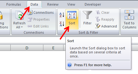
Select Data menu and select Sort from Sort & Filter group.

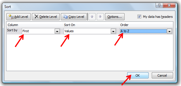
In the Sort by list, select the first column on which you want to sort. (You can click on Add Level to include additional number of columns to sort).
In the Sort On list, select the desired field from the drop down (ValuesCell ColorFont Color, or Cell Icon).
In the Order list, select the order that you want to apply to the sort operation (A to Z or Z to A for text, lower to higher or higher to lower for numbers).

Check the field My data has headers if your data has headers included.
Click OK.

Picture below shows the data after sorting.


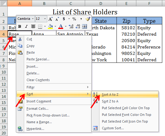
Method 2:

Select a single cell in the column of the range that you want to sort.
Right click on the selected cell and select Sort in the options appeared.
Select the desired options (A to Z or Z to A for text, lower to higher or higher

to lower for numbers).

Picture below shows the data after sorting.


————————————————————————————————————–

Vani is a Business Associate with p2w2, a Spreadsheet Solutions company. p2w2 has expertise in Excel ModelingExcel DashboardsProfitability Analysis,  Excel Invoicesand Excel Bid sheets. You can contact us by email: cs [at] p2w2.com or call us at 305.600.0950.
 

How to Use Conditional Formatting in Excel?

Conditional formatting is used to pick out important data from a huge list of data. Though it is a little difficult to use, knowing the basics can help us in whatever project we are working on.

We can use conditional formatting in many ways. Following are the two ways of using conditional formatting.

Conditional Formatting in Same cell
Conditional Formatting in Multi cell

Conditional Formatting in Same cell

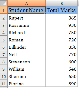
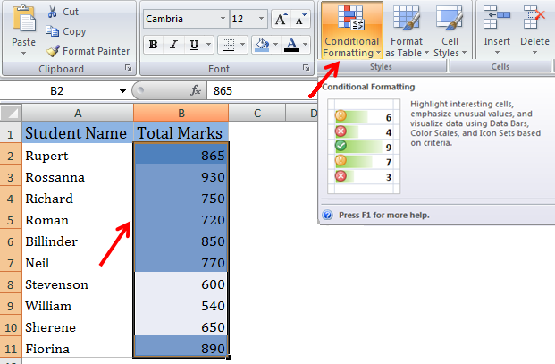
We can use this option, when we have to apply formats to the same cell. Let us take the example below to apply formats based on required conditions.

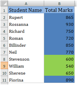
In column B of the above picture, the total marks of the students are displayed, we can identify the marks less than 700 and greater than 700 quickly by applying conditional formatting on column B.

Conditional formatting for the values Greater than 700.

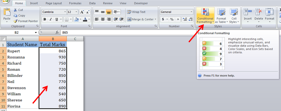
Select the cells to format and select Conditional Formatting from Home menu.

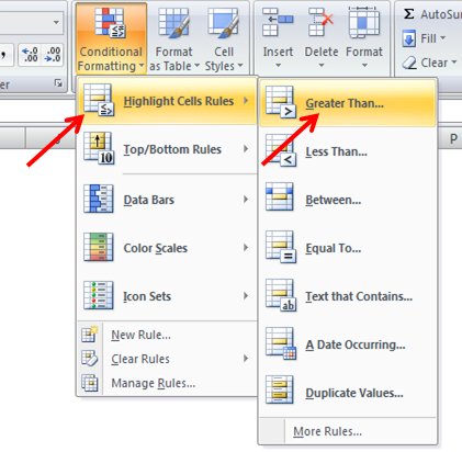
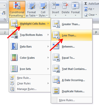
Select Highlight Cells Rules and select Greater Than from the drop down.

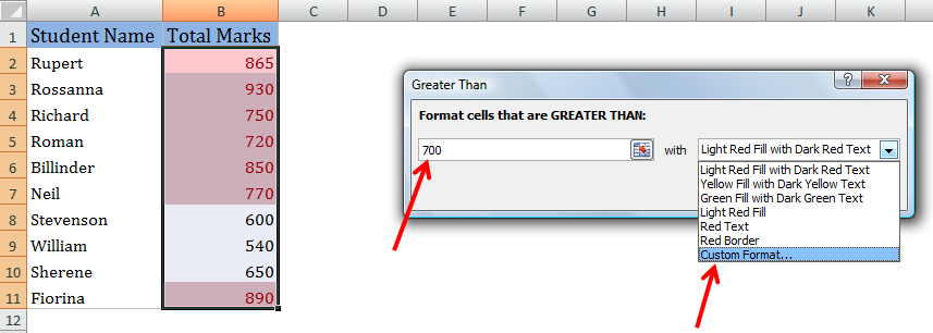
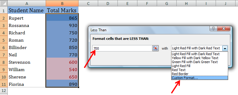
Enter the number in the box provided for “Format cells that are GREATER THAN:”, and select ‘Custom Format’.

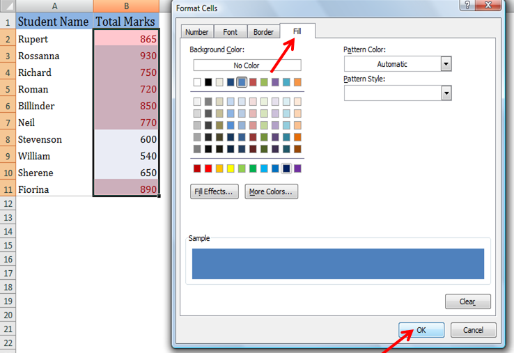
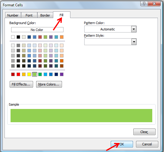
Select Fill from Format Cells, Select a required color from Background color and select OK.

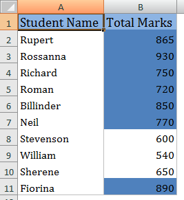
The picture shows the result after applying Conditional Formatting.


Conditional formatting for the values less than 700.

Select the cells which have to be formatted, select Conditional Formatting from Home menu,  Select Highlight Cells Rules and select Less Than.

Select the cells to format and select Conditional Formatting from Home menu.

Select Highlight Cells Rules and select Less Than from the drop down.

Enter the number in the box provided for “Format cells that are LESS THAN:”, and select ‘Custom Format’.

Select Fill from Format Cells, Select a required color from Background color and select OK.

The picture shows the result after applying Conditional Formatting.

Conditional Formatting in Multi cell

This option is used

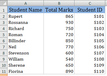
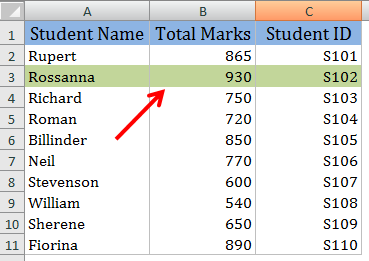
to apply formats to more than one cell based on one value. Let us take the example below to apply formats based on required conditions.

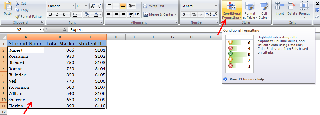
Select the cells to format and select Conditional Formatting from Home menu.

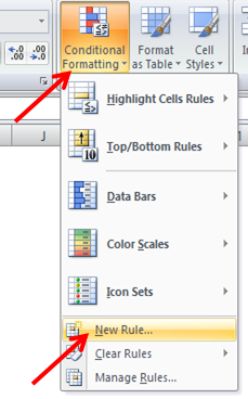
Select

New Rule from the menu.

Select Use a formula to determine which cells to format from New Formatting Rule window, enter the formula in the box provided for “Format values where this formula is true: , and select Format.

Select Fill from Format Cells, Select a required color from Background color and select OK.

The picture shows the result after applying Conditional Formatting.

————————————————————————————————————–

Vani is a Business Associate with p2w2, a Spreadsheet Solutions company. p2w2 has expertise in Excel ModelingExcel DashboardsProfitability Analysis,  Excel Invoicesand Excel Bid sheets. You can contact us by email: cs [at] p2w2.com or call us at 305.600.0950.