How to Sort in Excel?

Sorting is used to reorder our data in excel. We can easily reorder the data based on the type of sorting that we choose. We have two methods to sort the data.

Method 1:

Below are the steps to sort the given data in Excel:

Select a single cell anywhere in the range that you want to sort.
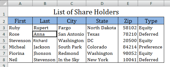
Note: If there are merged cells in your data, unmerge the cells before applying the Sort operation.

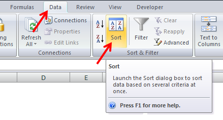
Select Data menu and select Sort from Sort & Filter group.
In the Sort by list, select the first column on which you want to sort. (You can click on Add Level to include additional number of columns to sort).
In the Sort On list, select the desired field from the drop down (ValuesCell ColorFont Color, or Cell Icon).
In the Order list, select the order that you want to apply to the sort operation (A to Z or Z to A for text, lower to higher or higher to lower for numbers).
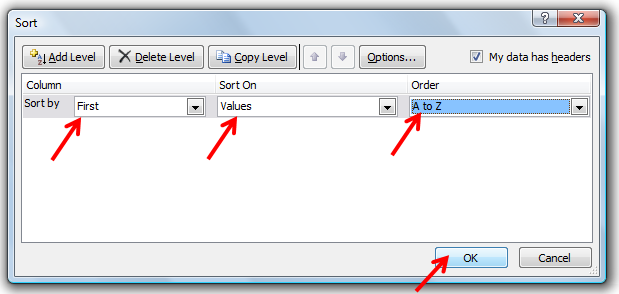
Check the field My data has headers if your data has headers included.
Click OK.

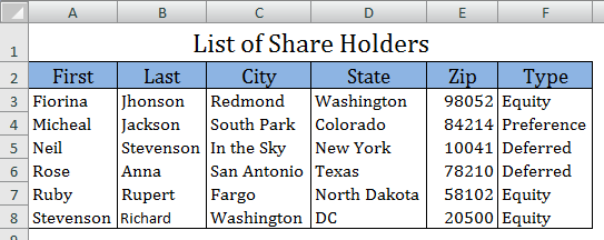
Picture below shows the data after sorting.
 

Method 2:

Select a single cell in the column of the range that you want to sort.
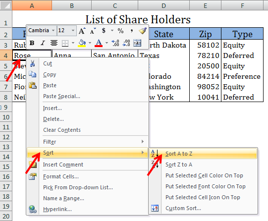
Right click on the selected cell and select Sort in the options appeared.
Select the desired options (A to Z or Z to A for text, lower to higher or higher

to lower for numbers).

Picture below shows the data after sorting.


————————————————————————————————————–

Vani is a Business Associate with p2w2, a Spreadsheet Solutions company. p2w2 has expertise in Excel ModelingExcel DashboardsProfitability Analysis,  Excel Invoicesand Excel Bid sheets. You can contact us by email: cs [at] p2w2.com or call us at 305.600.0950.


How to Use Conditional Formatting in Excel?

Conditional formatting is used to pick out important data from a huge list of data. Though it is a little difficult to use, knowing the basics can help us in whatever project we are working on.

We can use conditional formatting in many ways. Following are the two ways of using conditional formatting.

Conditional Formatting in Same cell
Conditional Formatting in Multi cell

Conditional Formatting in Same cell

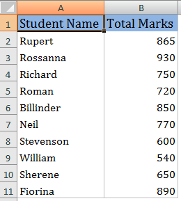
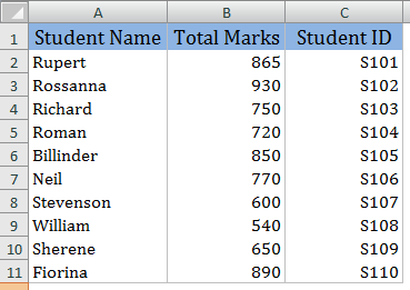
We can use this option, when we have to apply formats to the same cell. Let us take the example below to apply formats based on required conditions.

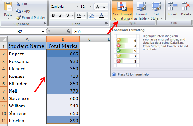
In column B of the above picture, the total marks of the students are displayed, we can identify the marks less than 700 and greater than 700 quickly by applying conditional formatting on column B.

Conditional formatting for the values Greater than 700.

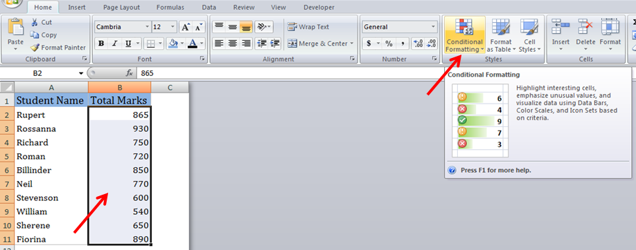
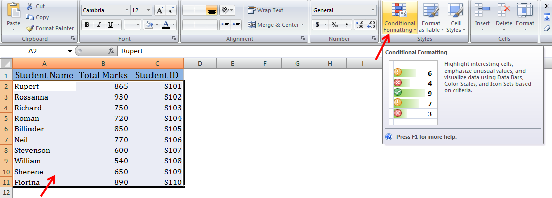
Select the cells to format and select Conditional Formatting from Home menu.

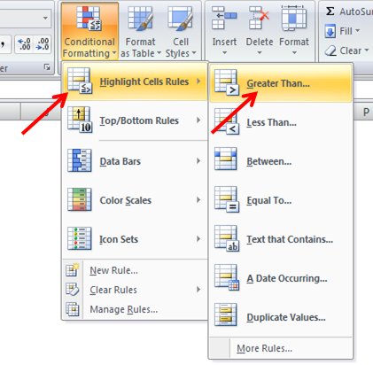
Select Highlight Cells Rules and select Greater Than from the drop down.

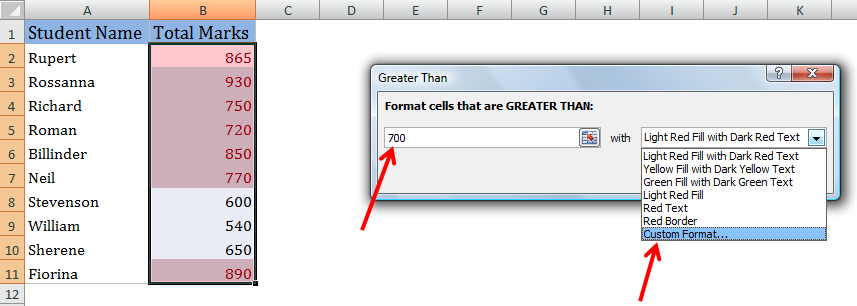
Enter the number in the box provided for “Format cells that are GREATER THAN:”, and select ‘Custom Format’.

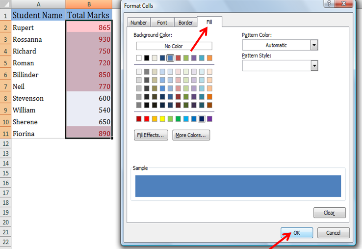
Select Fill from Format Cells, Select a required color from Background color and select OK.

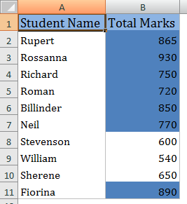
The picture shows the result after applying Conditional Formatting.


Conditional formatting for the values less than 700.

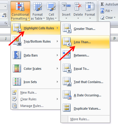
Select the cells which have to be formatted, select Conditional Formatting from Home menu,  Select Highlight Cells Rules and select Less Than.

Select the cells to format and select Conditional Formatting from Home menu.

Select Highlight Cells Rules and select Less Than from the drop down.

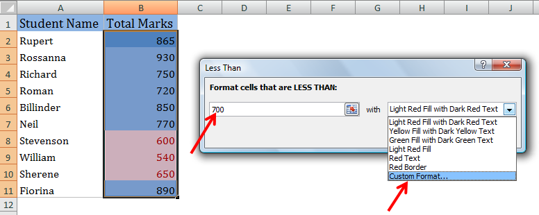
Enter the number in the box provided for “Format cells that are LESS THAN:”, and select ‘Custom Format’.

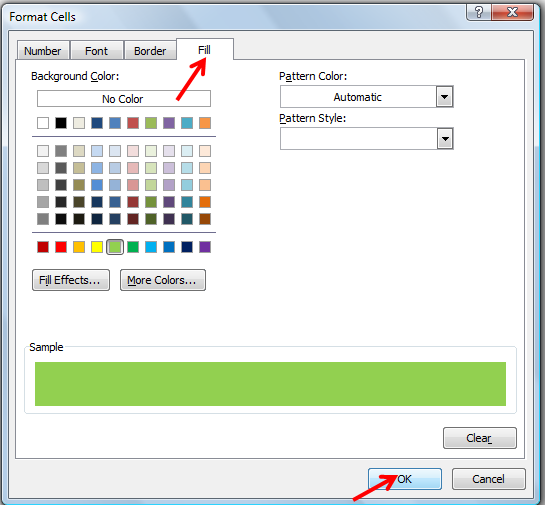
Select Fill from Format Cells, Select a required color from Background color and select OK.

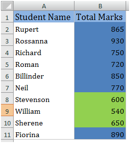
The picture shows the result after applying Conditional Formatting.

Conditional Formatting in Multi cell

This option is used

to apply formats to more than one cell based on one value. Let us take the example below to apply formats based on required conditions.

Select the cells to format and select Conditional Formatting from Home menu.

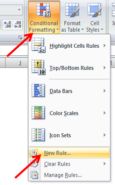
Select

New Rule from the menu.

Select Use a formula to determine which cells to format from New Formatting Rule window, enter the formula in the box provided for “Format values where this formula is true: , and select Format.

Select Fill from Format Cells, Select a required color from Background color and select OK.

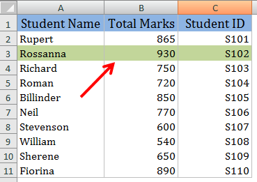
The picture shows the result after applying Conditional Formatting.

————————————————————————————————————–

Vani is a Business Associate with p2w2, a Spreadsheet Solutions company. p2w2 has expertise in Excel ModelingExcel DashboardsProfitability Analysis,  Excel Invoicesand Excel Bid sheets. You can contact us by email: cs [at] p2w2.com or call us at 305.600.0950.


How to Print Only Selected Objects in Excel?

Printing in Excel is a bit different than printing in some other programs, such as a word processor. Printing selected objects is one of the special features in Excel.

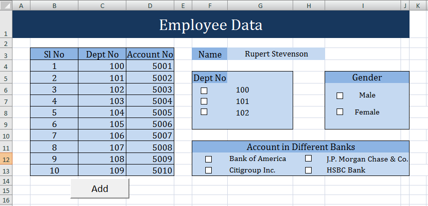
Worksheet with Objects.


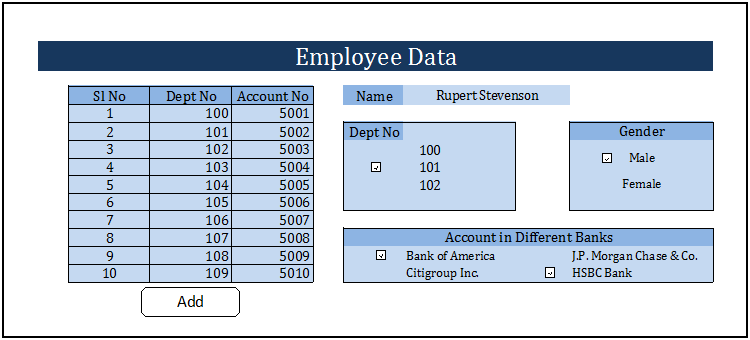
Print out with selected objects.

The steps below guide us to print only selected objects , from a number of objects (i.e. controls, images, shapes etc) in a worksheet.

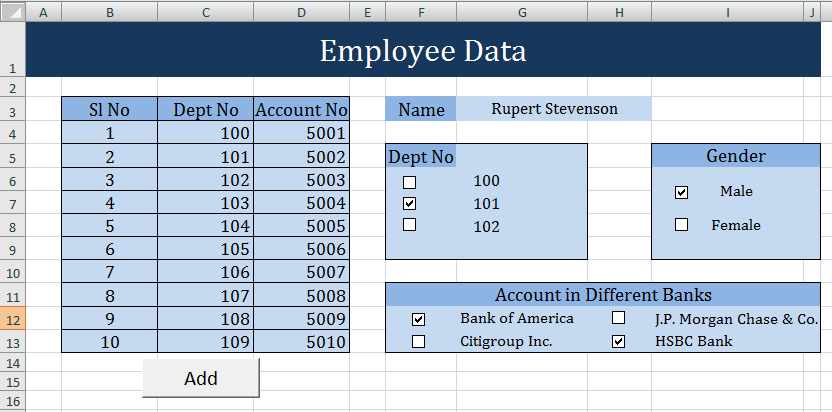
Select the required check boxes.


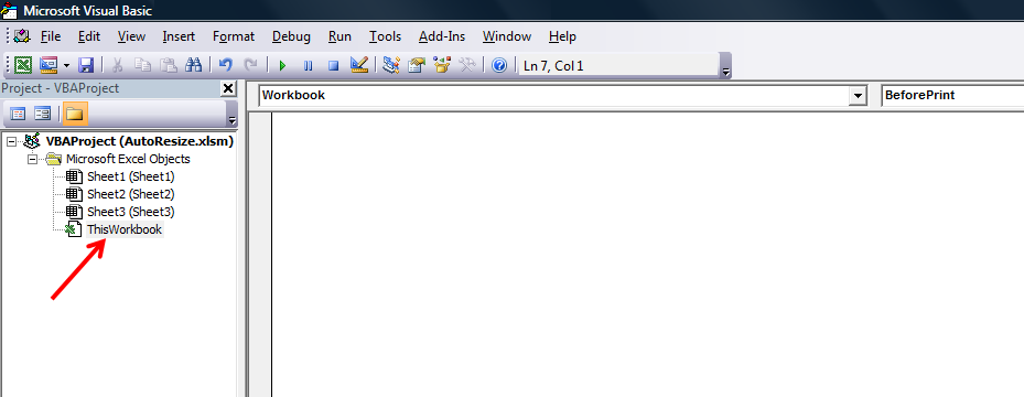
Press Alt+f11.

A ‘Microsoft visual basic‘ window appears.

Double click on ‘This Workbook’. The cursor appears in the space at the right

side, under the Workbook tab.

Now type the code below:

Private Sub Workbook_BeforePrint (Cancel As Boolean)

Dim CBX As CheckBox

For Each CBX In ActiveSheet.CheckBoxes

If CBX.Value = xlOff Then CBX.PrintObject = False

Next CBX

End Sub

After writing the macro, go to the worksheet and print the page, Now you can see the print out with selected objects only.


————————————————————————————————————–

Vani is a Business

Associate with p2w2, a Spreadsheet Solutions company. p2w2 has expertise in Excel ModelingExcel DashboardsProfitability Analysis,  Excel Invoicesand Excel Bid sheets. You can contact us by email: cs [at] p2w2.com or call us at 305.600.0950.